Loss attribution

The preceding guide asks how features account for a model’s prediction or class score. Loss attribution asks how features account for the change in prediction loss relative to the baseline, given an observed target. The second question builds on the first: keep the fitted model, reference inputs, and paths, and explain the model’s output after applying a loss function.

A different question

	Prediction attribution	Loss attribution
Question	What moves the prediction or class score relative to the reference?	What raises or lowers loss relative to the reference, for this target?
Function explained	The fitted model’s prediction or score	Loss evaluated on that output and the fixed target
Information required	Model, reference inputs, evaluation inputs	The same inputs, plus observed targets and a loss choice
Positive contribution	Increases the explained prediction or score	Increases loss in the default loss_change direction
Baseline value	Weighted mean reference prediction or score	Weighted mean reference loss, evaluated against this observation’s target

Prediction attribution can explain a model before the outcome is known. Loss attribution needs a target: a feature that raises the prediction can improve or worsen loss depending on what actually occurred. For classification, supporting one class on the score scale is a different statement from reducing log loss for the observed class.

Prediction changes and loss changes in a picture

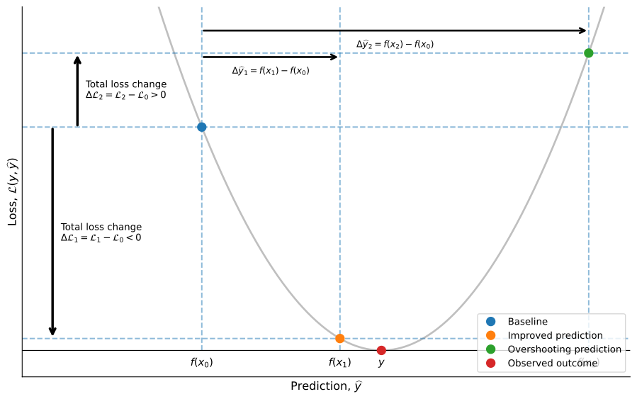
Prediction attribution decomposes the horizontal changes in model output. Loss attribution decomposes the corresponding vertical changes in loss, with the observed outcome \(y\) held fixed.

The blue point is the baseline prediction \(f(x_0)\). Moving to the orange point \(f(x_1)\) increases the prediction toward the observed outcome and lowers loss. Moving to the green point \(f(x_2)\) also increases the prediction, but overshoots far enough to make loss greater than at the baseline. Both horizontal prediction changes are positive; their total loss changes have opposite signs.

The graph shows output and loss differences, rather than individual feature allocations or an input-space path. Integrated Gradients distributes each of those totals across features using the baseline-to-observation paths. The slope of the loss curve supplies the additional derivative in the loss integral.

A complementary example holds the prediction change fixed and changes the target. Consider a one-feature model whose prediction rises from 2 at the baseline to 4 at the evaluation input. Its prediction contribution is +2 in both rows below. With squared-error loss, the target determines what that change means:

Observed target	Baseline loss	Endpoint loss	Loss contribution
5	(5 - 2)**2 = 9	(5 - 4)**2 = 1	-8: lower loss
1	(1 - 2)**2 = 1	(1 - 4)**2 = 9	+8: higher loss

The model and input path have not changed. Only the target changed, reversing the interpretation for model performance. In multiple dimensions, loss attribution allocates that total loss difference across input features.

These are decompositions of a fixed model’s behavior. A negative loss contribution does not establish that collecting that feature or retraining a model with it will improve performance. For performance analysis, use held-out observations and a reference population appropriate to the comparison.

Nearly the same calculation

Write the model output as f(x). For evaluation observation i, fix its target y_i and define the composed function g_i(x) = loss(y_i, f(x)). Prediction attribution integrates the input derivatives of f; loss attribution integrates the input derivatives of g_i along the same paths.

Using the same path \(\gamma(\alpha)=b+\alpha(x-b)\) as in prediction attribution, the scalar-output loss attribution is

\[ \mathrm{IG}^{\mathcal{L}}_j(x;b,y) = (x_j-b_j)\int_0^1 \frac{\partial\mathcal{L}}{\partial\widehat y} \bigl(y,f(\gamma(\alpha))\bigr)\, \frac{\partial f}{\partial x_j}\bigl(\gamma(\alpha)\bigr)\,d\alpha. \]

Relative to the prediction formula, there is one additional derivative inside the integral: how loss changes with the prediction. The target \(y\) remains fixed. In the default loss_change direction, contributions sum to \(\mathcal{L}(y,f(x))-\mathcal{L}(y,f(b))\). Weighted baseline distributions average these loss-path attributions just as they average prediction paths.

For smooth models the chain rule supplies the connection. If f has multiple score coordinates, their effects are combined through the loss derivative:

d g_i(x) / d x_j
    = sum_k [d loss(y_i, f(x)) / d f_k] * [d f_k(x) / d x_j].

For scalar squared error this reduces to:

d (y_i - f(x))**2 / d x_j
    = 2 * (f(x) - y_i) * d f(x) / d x_j.

The model derivative is the familiar prediction derivative. The extra factor measures how a change in output affects loss at each point along the path. It can change size and sign as the model prediction approaches or crosses the target. Loss contributions therefore cannot generally be obtained by multiplying finished prediction contributions by one endpoint error or slope. The loss must participate in the path calculation.

UnifiedIG reuses the underlying routes:

• skgrad: apply the loss chain rule to analytic model Jacobians and integrate along the same baseline paths.

• PyTorch, JAX, and TensorFlow: use native automatic differentiation on the composed loss, with the same path integration and batching infrastructure.

• Finite differences: estimate model derivatives numerically, then combine them with loss derivatives along the path.

• Exact TreeIG: reuse structural split crossings and account for the loss changes across prediction jumps. Ordinary smooth gradients alone would miss those jumps.

The fitted model is not retrained. Baseline normalization, weighted path averaging, feature-space selection, result containers, and completeness checks follow the prediction interface. Some numerical shortcuts and supported cases differ; the supported routes are listed below.

The same reference inputs, a target-specific reference loss

For observation i, UnifiedIG compares it with every baseline row b, retaining that observation’s target y_i along all paths. With normalized weights w_b, the default loss-change identity is:

base_loss_i = sum_b w_b * loss(y_i, f(baseline_b))
base_loss_i + sum_j loss_contribution_ij = loss(y_i, f(x_i)).

Thus the same shared baseline population can give different baseline losses for different evaluation observations. Baseline targets are not supplied or interpolated; the comparison is between model outputs evaluated against the same target for that observation.

As with nonlinear prediction attribution, averaging must respect the function being explained. The weighted mean of losses is generally different from the loss of the weighted mean prediction. A CBaseline distribution calibrated to a reference prediction remains a valid reference input distribution, but that calibration does not imply any particular reference loss.

From prediction attribution to loss attribution

The public calls make the change in question explicit:

prediction = uig.Explainer(model, background)(X_test)
loss = uig.LossExplainer(
    model, background, loss="squared_error"
)(X_test, y_test)

Keep background and the attribution feature space fixed if you want to compare the two explanations. Interpret their values in different units: prediction units versus squared prediction units for squared error, or scores versus log loss for classification. Both return an Explanation, with baseline values and a completeness residual for their own explained function.

Squared-error loss

import numpy as np
from sklearn.linear_model import Ridge

import unifiedig as uig

rng = np.random.default_rng(0)
X = rng.normal(size=(240, 3))
y = 2.0 * X[:, 0] - X[:, 1] + rng.normal(scale=0.5, size=len(X))

model = Ridge(alpha=0.5).fit(X[:160], y[:160])
background = X[:40]
X_test, y_test = X[160:], y[160:]

explanation = uig.LossExplainer(
    model,
    background,
    loss="squared_error",
)(X_test, y_test)

np.testing.assert_allclose(
    explanation.base_values + explanation.values.sum(axis=1),
    (y_test - model.predict(X_test)) ** 2,
)

The default direction is loss_change. Contributions sum to endpoint loss minus baseline loss: negative values reduce loss and positive values increase it. The observed target for each evaluation row is held fixed along every path. Consequently, baseline loss can differ by observation even for a shared baseline population. It is the weighted mean of baseline losses, not the loss of the weighted mean baseline prediction.

Binary and multiclass log loss

Use loss="log_loss" with a classifier supplying raw scores. Targets must be valid class labels (or the adapter’s supported class indices for framework models). The score-based loss reconstructs binary or multiclass log loss.

import numpy as np
from sklearn.linear_model import LogisticRegression

import unifiedig as uig

rng = np.random.default_rng(4)
X = rng.normal(size=(300, 4))
scores = np.column_stack((X[:, 0], X[:, 1], -X[:, 0] - X[:, 1]))
y = np.argmax(scores + rng.normal(scale=0.5, size=scores.shape), axis=1)

model = LogisticRegression().fit(X[:200], y[:200])
background = X[:50]
X_test, y_test = X[200:], y[200:]

explanation = uig.LossExplainer(
    model,
    background,
    loss="log_loss",
)(X_test, y_test)

endpoint_loss = -np.log(model.predict_proba(X_test)[np.arange(len(y_test)), y_test])
np.testing.assert_allclose(
    explanation.base_values + explanation.values.sum(axis=1),
    endpoint_loss,
    atol=2e-9,
)

Present improvements as positive numbers

direction="loss_reduction" negates the returned feature contributions only. In that presentation, positive values improve loss and the reconstruction is:

endpoint_loss = result.base_values - result.values.sum(axis=1)

Baseline values and completeness diagnostics retain the original loss-change convention. Use this subtraction only for the loss-reduction direction.

Supported routes and controls

Loss attribution supports scalar squared-error regression and binary or multiclass log loss through skgrad, exact TreeIG, native PyTorch/JAX/TensorFlow, and the explicit finite-difference backend. The numerical tree detector does not supply a loss backend. Multi-output regression loss is not supported.

Baseline distributions and attribute_after follow the prediction interface. The usual integration and completeness controls apply; affine squared-error loss uses one exact node, while affine log loss starts with eight nodes when resolution is automatic. See the API for all parameters.