Attribution and interpretation

Why TreeIG?

The method is developed in Ludger Hentschel’s TreeIG: Exact Integrated Gradients for Tree-Based Models. It builds on Integrated Gradients introduced by Sundararajan, Taly, and Yan in Axiomatic Attribution for Deep Networks (ICML 2017).

Standard Integrated Gradients defines feature contributions by integrating model gradients along a straight-line path from a baseline input to the observation. Tree models are piecewise constant, so ordinary gradients are zero almost everywhere and undefined at split boundaries.

TreeIG uses the tree structure directly. Along the interpolation path

\[ x(t) = x_0 + t\,(x - x_0),\qquad 0 \le t \le 1, \]

a tree prediction changes only when the path crosses a split threshold. TreeIG finds those crossings exactly and assigns each prediction jump to the feature responsible for the crossing. For ensembles, contributions are summed across trees. The result is an exact additive decomposition without numerical quadrature.

The distributional-derivative perspective makes this precise. Along the interpolation path the prediction is piecewise constant, and its generalized derivative is a sum of localized impulses at split crossings. The path integral of each impulse is exactly the prediction jump at that crossing.

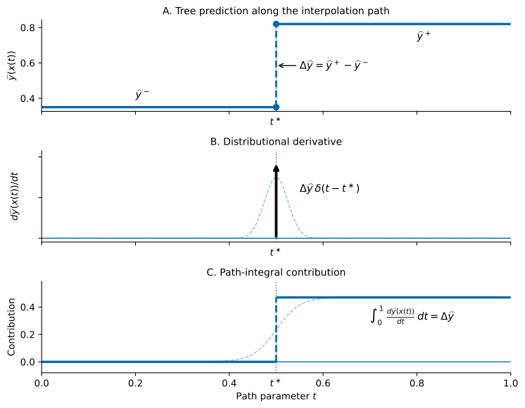
The top panel shows a step in the tree prediction along the interpolation path. The middle panel shows the corresponding distributional derivative: zero everywhere except at the split crossing. (Here, \(\delta(t - t^\ast)\) is the Dirac delta distribution centered at \(t^\ast\).) The bottom panel shows that the path integral localizes exactly at the crossing and recovers the prediction jump. TreeIG exploits the fact that integrated gradients applied to trees requires neither numerical differentiation nor numerical integration; it reduces to a simple sum of prediction steps along the integration path \(x(t)\).

Standard numerical Integrated Gradients methods try to approximate these impulses using dense interpolation grids. TreeIG instead computes the split-crossing contributions analytically from the fitted tree structure. In this sense, TreeIG plays a role analogous to automatic differentiation for smooth models: rather than numerically searching for discontinuities, it uses the model’s computational structure to evaluate the attribution integral exactly and efficiently. (The analogy understates the gain. Automatic differentiation removes derivative approximation but not the numerical quadrature used by Integrated Gradients. TreeIG exploits tree structure to evaluate the attribution integral itself exactly.)

Crossing boundaries in two dimensions

The same principle applies when a path crosses splits on different features. The figure below follows a straight path from baseline \(x_0\) to observation \(x\).

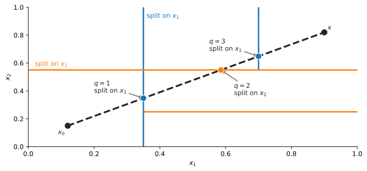
Boundary crossings along a baseline-to-observation path. The index \(q\) numbers crossings in path order. Blue boundaries split on \(x_1\); orange boundaries split on \(x_2\). The prediction jumps at crossings 1 and 3 contribute to \(x_1\), while the jump at crossing 2 contributes to \(x_2\). Boundaries not crossed by the path make no contribution. Contribution size is the signed prediction jump, not the distance traveled; leaf prediction values are not shown.

Writing the signed jump at crossing \(q\) as \(\Delta F_q\), this example gives

\[\phi_1 = \Delta F_1 + \Delta F_3,\qquad \phi_2 = \Delta F_2.\]

Their sum is \(F(x)-F(x_0)\). For an ensemble, TreeIG adds these contributions across trees; for a baseline distribution, it averages them across baseline paths with the supplied weights.

Interpretation

For an observation \(x\), TreeIG reports how much each feature contributes to moving the model output from \(F(x_0)\) to \(F(x)\) along the straight-line path from \(x_0\) to \(x\). Positive contributions increase the scalar output relative to the baseline; negative contributions decrease it. The contributions are additive by construction.

Numerical conventions

TreeIG follows each backend’s split-routing convention as closely as possible.

• scikit-learn trees route left when x[j] <= threshold;

• LightGBM numeric splits route left when x[j] <= threshold;

• XGBoost numeric splits route left when x[j] < threshold using float32-style comparisons.

XGBoost completeness comparisons against native raw predictions can show small residuals (around 1e-7 in tested models), consistent with differences in floating-point precision and accumulation between the native predictor and the attribution calculation. This is not a universal error bound or a numerical integration resolution; compare residuals relative to the scale of the explained output.

Inputs must be finite numeric arrays. Missing-value routing is not currently implemented, so NaN and Inf values raise errors.

Endpoints and simultaneous crossings

Endpoints use the fitted backend’s routing convention. A baseline or observation exactly on a split can therefore contribute an endpoint jump. Keep this behavior in mind when constructing synthetic examples near thresholds: nearby decimal inputs may map to the same float32 value in a backend that rounds inputs.

The current tie_policy="first" assigns a coincident effect to the first divergent split feature. Other policies are not implemented. Completeness checks the total allocation, not whether a different tie convention would assign it to the same features. time_tol controls crossing comparisons; it is not a user-selected numerical integration resolution.

These are explanations of a fitted model along specified paths. They do not, by themselves, establish causal effects. A straight path can pass through input combinations that are unusual in the training data.