CBaseline documentation#
CBaseline is a Python package that constructs empirical reference background
distributions for Integrated Gradients, SHAP, and other compatible attribution
methods. Install and import it as cbaseline. Given aligned model predictions,
a reference output f0, and observed feature rows, background(...) returns
selected rows, weights, and diagnostics. Your attribution engine then computes
the feature contributions.
Attribution methods explain a contrast. CBaseline constructs the reference population that defines it.
Integrated Gradients and Shapley attribution both decompose \(f(x)-f_0\) for some reference output \(f_0\). That reference is usually inherited rather than chosen. An all-zeros baseline generally lies off the data manifold. A mean input \(\bar{x}\) is not an observed case, and for nonlinear \(f\), \(f(\bar{x}) \neq \mathbb{E}[f(X)]\), so the corresponding reference output is not the mean prediction.
A useful reference must satisfy two separate requirements. It must be neutral — its mean model output equals \(f_0\) — and it must be localized — assembled from cases the model already predicts near \(f_0\). With a background distribution \(Q\), complete attributions explain \(f(x)-\mathbb{E}_Q[f(X)]\), so neutrality is the condition \(\mathbb{E}_Q[f(X)]=f_0\).
CBaseline satisfies both using observed rows only. It localizes in prediction space under a fitted metric that accounts for output scale and redundant directions, then calibrates by exponential tilting until the weighted mean output equals \(f_0\) to numerical tolerance. Equal-weight backgrounds approximate neutrality with a fixed-size selection and report the residual they achieve.
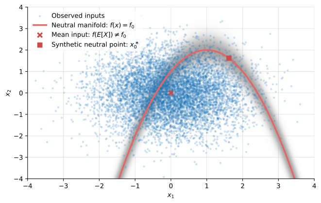
The blue points are observed inputs; the red curve is the neutral manifold, \(\mathcal{M}_0=\{x:f(x)=f_0\}\). CBaseline builds its background from observed cases near this curve in prediction space, illustrated by the shaded band. The background therefore represents realistic reference inputs concentrated around the prediction being used for comparison.
The construction is method-agnostic. The same background serves Integrated Gradients, interventional Shapley attribution — where the weighted mean is the empty-coalition value \(v(\emptyset)\) — and any implementation that accepts a background matrix. Calibrated weighted backgrounds fit naturally into the UnifiedIG / TreeIG stack. Deterministic equal-weight backgrounds give SHAP a first-class workflow through its standard background-matrix interfaces.
See prediction-neutral backgrounds for why both requirements are needed and how they constrain one another.
Choose a background#
Attribution workflow |
Mode |
What neutrality means |
|---|---|---|
An engine that accepts observation weights, such as UnifiedIG or TreeIG |
|
The weighted mean prediction meets configured tolerances around |
A standard SHAP background-matrix interface |
|
A deterministic fixed-size subset approximates |
Localization without enforcing neutrality |
|
Kernel weights favor predictions near |
Preserve both rows and weights for weighted attribution. Calibrated targets
must be supported by the available predictions; an arbitrary f0 is not always
feasible. For every mode, the attribution reference is the achieved background
mean, and predictions must use the same output scale as the attribution engine.
The supporting papers#
Hentschel (2026a), Canonical Integrated Gradients: Expectations over Neutral Prediction Baselines: the reference-distribution formulation and calibrated estimation.
Hentschel (2026b), A Canonical Background Distribution for Shapley Attribution: the Shapley formulation and equal-weight construction.
The guide develops the practical ideas alongside the papers; see papers and citation for BibTeX and further reading.
Where to start#
Background modes and diagnostics explain feasibility, residuals, and failure behavior. For automated readers, llms.txt maps the guides, complete examples, and rendered API reference.
Use getting started for a runnable construction, integrations for attribution examples, and choosing the reference prediction before adapting an example to classification.